Backpropagation answers a practical question: if the prediction is wrong, which weights caused the mistake, and how much should each one change?
This guide builds the idea from the ground up. We start with one neuron, then a two-layer network, and finally the vectorized version used in real training. We keep the math honest, but we explain it in plain English.
If you can follow this article, you will be able to read gradient code, debug shape errors, and understand why modern frameworks compute gradients the way they do.
Training is just loss reduction. You have a number that says how wrong the model is, and you want to push that number down.
To do that, you need a direction for every parameter. That direction is the gradient: how the loss changes if a weight moves a tiny amount.
Backpropagation is the algorithm that computes all those gradients efficiently in one backward sweep.
Take a single neuron with input x, weight w, bias b, activation a = f(z), and z = w x + b.
Let the loss be L = (a - y)^2. We want dL/dw. The chain rule lets us break it into small pieces.
L = (a - y)^2
a = f(z)
z = w x + b

dL/da = 2(a - y)
da/dz = f'(z)
dz/dw = x

=> dL/dw = 2(a - y) * f'(z) * x
That is the pattern you will see everywhere: incoming gradient times a local derivative.
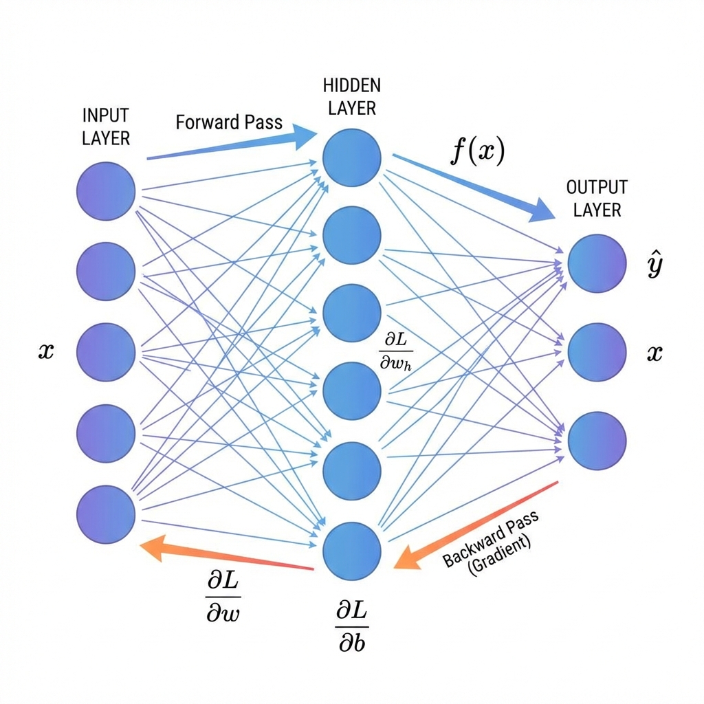
A computational graph is a picture of the computation. Each node stores its output and knows how to compute its local derivative.
Backprop walks the graph backwards. At each node you multiply the gradient you already have by that node's local derivative.
Now scale up to a small but realistic model: one hidden layer, a nonlinearity, and a softmax output.
We will track shapes because most backprop bugs are shape bugs.
x: (d, 1)
W1: (h, d), b1: (h, 1)
W2: (k, h), b2: (k, 1)

z1 = W1 x + b1
a1 = sigma(z1)
z2 = W2 a1 + b2
y_hat = softmax(z2)
L = -sum(y * log(y_hat))
Store z1, a1, z2, y_hat. You will reuse them in the backward pass.
Start at the loss and move backward. For softmax with cross-entropy, the first gradient is simple.
dz2 = y_hat - y
dW2 = dz2 * a1^T
db2 = dz2

da1 = W2^T * dz2
dz1 = da1 * sigma'(z1)
dW1 = dz1 * x^T
db1 = dz1
Each gradient has the same shape as its parameter. Use that as a constant sanity check.
In real training you use batches. Replace vectors with matrices and do the same math in parallel.
Let x be (d, m). Then z1 and a1 are (h, m), and z2 is (k, m).
dW2 = (1/m) * dz2 * a1^T
dW1 = (1/m) * dz1 * x^T
Averaging by m makes learning rate behavior stable as you change batch size.
Softmax followed by cross-entropy collapses to a clean gradient: y_hat - y. That is why most classification models use this pair.
This simplification reduces numerical error and makes the backward pass fast.
If you implement backprop by hand, verify it. Compare your analytic gradients with finite differences.
grad_approx = (L(theta + eps) - L(theta - eps)) / (2 * eps)Do this on a tiny model. If relative error is around 1e-6 to 1e-4, you are usually correct.
Softmax stability: subtract max before exp
Gradient clipping for exploding gradients
He/Xavier initialization to reduce vanishing gradients
Normalize inputs so activations stay in a healthy range
These are not hacks. They are fixes for numerical issues that appear in real systems.
Print shapes at every layer
Overfit a tiny dataset first
Check gradients for NaNs
Validate with gradient checking
Try it
In a two-layer network with softmax + cross-entropy, what is dL/dz2?
Put the backward pass steps in the correct order.
Drag and drop practice coming soon! For now, here are the items to match:
Which is the most reliable quick check for gradient shapes?
Backpropagation is the chain rule organized for efficiency. Once you understand local derivatives and cached activations, the full algorithm feels predictable.
Implement the two-layer example, pass gradient checking, and you will have the confidence to build deeper models and debug them when they misbehave.