Machine learning is optimization. Calculus is the tool that tells you how to move your parameters to make the loss go down.
This article is a practical bridge between calculus and ML. We will focus on the ideas you actually use: limits, derivatives, gradients, the chain rule, and why gradient descent works.
No heavy jargon. Just clear explanations, small examples, and the intuition you need to debug real training code.
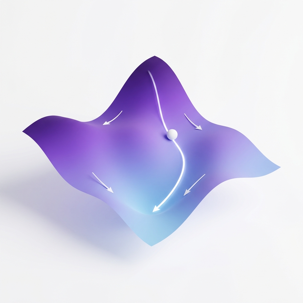
Training means minimizing a loss function. The loss is a surface over all parameters. Calculus tells us which direction reduces that loss.
Even when the surface is high‑dimensional and messy, the local slope still gives useful guidance.
A derivative is defined using a limit. It measures how a function changes when the input changes by a tiny amount.
f'(x) = lim_{h→0} (f(x+h) - f(x)) / hIn ML, this tiny change is the small step you take in parameter space.
A derivative is slope. If the slope is positive, moving right increases the loss. If it is negative, moving right decreases the loss.
Gradient descent simply moves in the opposite direction of the slope.
Models have many parameters. You need a slope for each one. That is a partial derivative.
∇L = [∂L/∂w1, ∂L/∂w2, ..., ∂L/∂wn]The gradient vector points uphill. We move downhill by subtracting it.
Locally, any smooth function looks linear. This is the key idea behind gradient descent.
If you take a small step opposite the gradient, the loss will usually go down.
w = w - lr * ∇L(w)Neural networks are functions of functions. The chain rule is what lets us compute derivatives through that stack.
Backprop is just the chain rule applied efficiently to every parameter.
If y = f(g(x)), then dy/dx = (dy/dg) * (dg/dx)The Jacobian generalizes gradients when outputs are vectors. The Hessian captures curvature.
Most ML code does not compute Hessians directly, but it helps to know that curvature affects how fast you can learn.
If the learning rate is too large, you overshoot. Too small, and training crawls.
Schedules, warmup, and adaptive optimizers are all ways to manage this trade‑off.
Regularization adds a penalty term to the loss. That changes the gradient and pulls parameters toward smaller values.
L2 adds λ||w||^2, L1 adds λ|w|. The derivatives of those penalties are simple and easy to implement.
Overfit a tiny dataset to test your pipeline
Plot loss curves to spot learning‑rate issues
Watch for NaNs and exploding gradients
Try it
What does the gradient vector point toward?
Order the steps of gradient descent.
Drag and drop practice coming soon! For now, here are the items to match:
Which statement about learning rate is correct?
Calculus is the engine behind machine learning. Limits define derivatives, derivatives form gradients, and gradients drive optimization.
Once you connect those ideas to training code, the math stops feeling abstract and starts feeling like a practical tool.